CORRELATION AND REGRESSION
CORRELATION
In this section we will first see the need for studying correlation and then learn how to calculate Correlation Coefficient with an example. Finally we will compare the two approaches and discuss how one can take best advantage of both by using them in combination.
Need for Correlation
In process control one aims to control the characteristics of the output of the process by controlling a process parameter. One succeeds in this if the parameters are correctly chosen. The choice is usually based on judgement and knowledge of the concerned technology. One assumes correlation between a variable product characteristic and a variable process parameter. There is a need to test if the assumption is correct particularly when one gets nonconforming output inspite of the process appearing to be in control. This is why one needs to study the correlation between the two variables. Scatter diagrams describe the correlation graphically and in qualitative terms like positive or negative and strong or mild relationship. In the next section we will see how to describe the relationship quantitatively.
CORRELATION COEFFICIENT
The quantitative measure of correlation between two variables, the correlation coefficient, is represented by the symbol r. To calculate value of r, one needs several paired observations. The formula for calculating r is
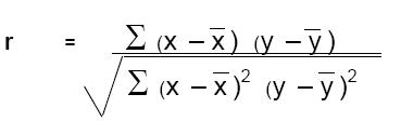
There is an alternate formula which at first appears more complicated but in practice is a little easier to use.
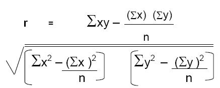
Today one rarely needs either of these as computer programmes are available which calculate the value of r if one keys in the paired values of x and y. Even pocket calculators with statistical functions are programmed to calculate r from paired values of x and y.
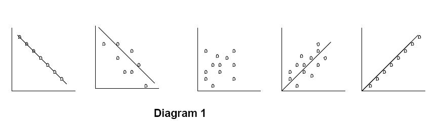
The total range of the value of is – 1 to + 1. A score of –1 indicates a very strong negative relation meaning that if x goes up y goes down proportionately and vice versa. A score of + 1 indicates a strong positive relationship where both x and y go up or down together. A score of 0 indicates an absence of relationship. Values closer to 0 than to 1 indicate relatively mild relationship and values closer to 1 indicate stronger relationship. All positive values indicate direct relation and all negative values indicate inverse relation. Diagram 1 explains this graphically.
EXAMPLE
It is believed that the purity of a chemical produced is related to the temperature at which the reaction was carried out. A need was felt to test the correlation between the two variables – process parameter (reaction temperature) and the product characteristic (purity). Ten experiments were conducted. The results of the experiments are provided in table 1 in the form of ten sets of paired data.
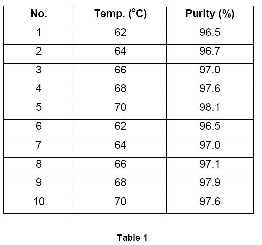
To calculate the correlation coefficient r, we have to first calculate the squares and the product of the individual values of variables x (temperature) and y (purity) and their sums. These are provided in Table 2.
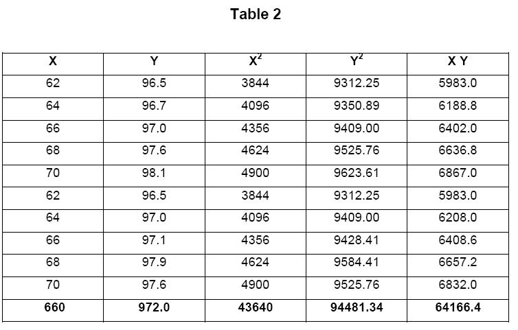
The correlation coefficient is now calculated using the numbers in Table 11.2
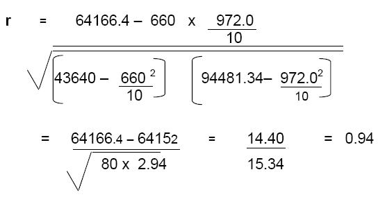
As the value of r is positive, one concludes that the relation between the two is positive meaning that the purity improves with higher reaction temperature and goes down with lower temperature. The value is very close the maximum possible value of 1 and hence the relation is very strong.
REGRESSION
While calculating correlation coefficient, also called regression coefficient ( r). The data was fitted into a best fitting straight line. The formula that describes this straight line has some constants. These constants help one predict the value of one variable for a given value of the other. Thus one can use it to predict the value of a product characteristic for a given value of a process parameter. The constants can also be used to decide a value of the process parameter that will result in a desired value of the product characteristic. These are the two major uses of regression. We will now see how to calculate the constants that describe the best fitting straight line and then see how the constants are used to predict results and to optimize the process.
Calculation of Constants
In school algebra, one learnt to solve problems where something was partly constant and partly variable with another thing. The formula used was “y = mx + c”. This is a standard formula that represents a straight line. This formula is used in regression with the only difference that conventionally symbols a and b are used for the constants instead of m and c. Thus the formula commonly used in regression is “y = ax + b”. The value of a and b are calculated using the following formula which involves the same data as that used for calculating the correlation coefficient r.
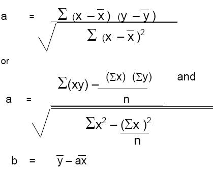
As mentioned during the discussion in the calculation of r, the second formula for calculating a, though appearing more complicated, is simpler to use. Let us calculate the constants a and b for the data provided in Table 11.1 The calculations presented in Table 2 are useful in calculating the value of a also. Thus
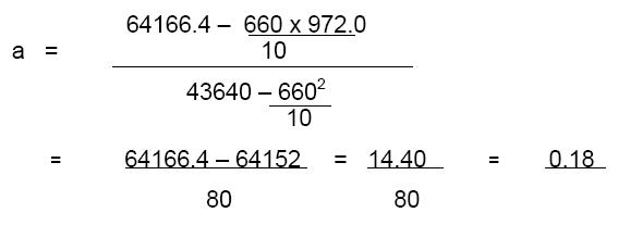
once the value of a is calculated, the calculation of the value of b is very simple.
b = 97.2 – 66.0 x 0.18
= 97.2 – 11.88 = 85.32
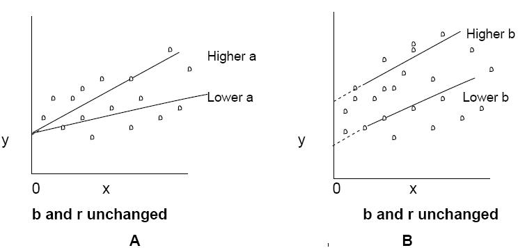
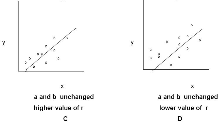
In this chapter, we have learnt to calculate the value of three constants – a, b and r- from a given set of paired data. To get a total understanding of correlation and regression it is necessary to understand the importance of these three and their impact on the straight line that best fits the data. The constant a relates to the slope of the line which decides the extent of change in y with unit change in x. The constant b indicates the point where the line, if extended, will cross the y-axis. In other words, b = y when x = o. r shows how closely the individual data points on the graph fit the line. To get a grasp of this we will see, in Diagram 4, the effect of change in only one of them with the other two remaining unchanged.
In Diagram 4 A, as b and r are unchanged the point of intersection of y-axis by the line and the clustering of the points around the line are the same. The effect of change in a is seen in the slope of the line i.e. its angle with respect to the x-axis. In Diagram 4 B, as a and r are unchanged the slope of the line and the distribution of the points around the line remain the same but because of the difference in the value of b, the line touches y-axis at a different point. For showing the impact of change in the value of r we need two separate diagrams – Diagrams 4C and 4 D. As both a and b are the same the line remains exactly the same but the scatter of the points is closer to the line when the value of r is higher.
PREDICTING RESULTS
Now that we have learnt how to calculate the value of a, b and r and understood the importance and the effect of each of them, let us see how one can use these constants in predicting the result or the product characteristic for a fixed value of the process parameter i.e. the value of y for a given value of x. The formula used for calculating the value of y is – y = ax + b. In the example seen earlier, the values of a and b were 0.18 and 85.32. If we want to predict the % purity of the output with the reaction temperature fixed at 65oC, we can calculate it using the formula.
Y = 0.18 x 65 + 85.32 = 97.02
Thus the prediction is that if the reaction temperature is 65oC, the purity of the output will be 97.02%. The value of r has not come into this calculation. Thus value of r does not affect the value of y. However, it affects the accuracy of the prediction. The actual value of y will be very close to the calculated value if the value of r is nearer to +1 or –1 but not so close if the value is nearer to 0. Thus values of a and b impact the predicted value of y and the value of r impacts the accuracy of the prediction. We have seen in an earlier section that grouping the data and calculating r for linear portions of the scatter diagrams would result in a better fitting line and a higher value of r. Thus using scatter diagrams and correlation coefficient in an ideal combination discussed in that section will improve the accuracy of prediction of results. This is also applicable to the optimization of the process parameters.
OPTIMISING A PROCESS
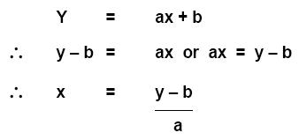
Optimising the process is the reverse of prediction of results. For predicting results, one has to calculate the value of y for a given value of x. For optimizing the process, one needs to calculate the value of x for getting a desired value of y. In other words, it involves calculating the optimum value of process parameter to get the desired value of the product characteristic. The formula ‘y = ax + b’ still applies but we will have to change its base to derive the formula to be used.
Continuing with the same example, let us say one wants to find the reaction temperature that would result in 97.5% purity of the output. The value of x will be calculated as
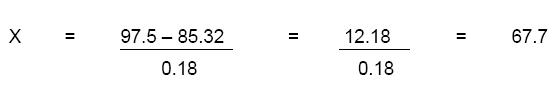
Thus, one fixes the reaction temperature at 67.7oC if the purity desired is 97.5%. A question is likely to arise ‘why should one desire a purity of only 97.5%, why not 100%?” There are two reasons for this – one statistical and the other technical. Statistical reasoning is that linearity of the relationship applies to only the range covered by the data. One may have to collect additional data to check if the yield improves when the temperature goes higher than 70oC. The chemist probably knows that ideal temperature is in the range of 62 to 70oC and hence the temperature was kept limited to that range in the experiments. It is possible that the reaction may produce undesirable by products if the temperature goes above 70oC. Hence it is not safe to go beyond that temperature. One must remember that statistical tools are aids to the technician to be used in combination with his knowledge about his own scientific discipline. The tools are not substitutes for technical judgement.